Quickstart Guide

This is intended as a quick guide for people already familiar with GPI and the original gpilib to get up and running with gpilib2. For all others, it is strongly recommended that you read the rest of this documentation before running the instrument.

Note

All code blocks in this page are intended to be executed inside a python interactive session (and preferably an ipython session). Some code blocks also include sample outputs from running certain commands.

gpilib2 Objects

In normal operation, the main entry point to instrument control is via the instantiation of a gpi object:

import gpilib2.gpi
gpi = gpilib2.gpi.gpi()

The initialization of a gpi object automatically generates multiple other objects (as shown in Fig. 1), which are all set as its attributes. Each of these objects groups together similar mechanisms or similar functionality. Frequently this corresponds to a single GPI assembly (for example, the powerbars object exactly maps to the powerbar assembly). In other cases, commands from multiple assemblies are bundled together (for example, the coronagraph object bundles the apodizer, FPM, and Lyot, and thus calls commands from the PPM, FPM, and IFS assemblies).

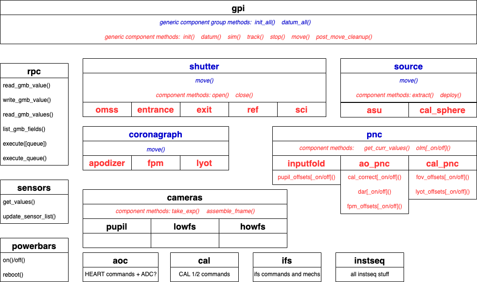
Fig. 1 gpilib2 classes. All sub-blocks are object attributes of a parent object and all individual blocks are attributes of the top-level gpi object.

Any and all of the objects generated by creating an object instance of gpi can also be instantiated on their own (i.e., you can always create a bare instance of coronagraph), but there is typically no reason to do so, other than for code debugging tasks.

The rpc Object

The first object instantiated when initializing gpi is rpc. This is then passed to the __init__ methods of all other objects. rpc is the main means of communicating with the instrument and includes utility methods for reading and writing GMB fields and sending commands via RPC calls. The rpc is essentially a thin wrapper for a large number of binaries, whose location on disk is stored in the internal dictionary binaries. It is possible to create multiple different rpc objects within a single session (and you could actually use a separate object for each separate sub-class generated by building a gpi object, but, again, in normal usage there is seldom reason to do so.

The rpc object determines whether you are operating the actual instrument or running in a simulated mode (set by the boolean attribute sim and as an input to the __init__ of both rpc and gpi.

Note

The gpilib2 is distinct from the built-in SIM capabilities of GPI itself. When rpc are created wit sim=True, no commands are actually sent to the instrument at all, and all instrument responses are simulated.

In order to create a simulated interface, run:

import gpilib2.gpi
gpi = gpilib2.gpi.gpi(sim=True)

The rpc object also has a verbose mode, toggled by verb and as an input to the __init__ of both rpc and gpi. Verbosity can be toggled on and off at any time by running:

gpi.rpc.verb = True

and

gpi.rpc.verb = False

Note

Creating the rpc with sim=True will automatically set verb=True as well. This can then be turned off, by using the command above, if so desired.

Getting Information

All gpi sub-objects have helpful __str__ methods, such that calling print on them will display useful information. For example:

print(gpi.powerbars)

will show the current powerbar status, like so:

------------------------------------------------------------------------------------------------
|                          1|                   2|                     3|                     4|
------------------------------------------------------------------------------------------------
|1|         IFS_COMPUTER: ON|        IFS_CCRS: ON|      TLC_COMPUTER: ON|          OMSS_PZT: ON|
|2| IFS_SERIAL_PUPIL_CAM: ON|     IFS_GALIL_2:OFF| SPARE_PB3_OUTLET2:OFF|               GIS: ON|
|3|     AVCS_ELECTRONICS:OFF|     CAL_SHUTTER: ON|  AOC_PCI_EXTENDER: ON| SPARE_PB4_OUTLET3:OFF|
|4|    CAL_OMSS_SERIAL_2: ON| SUPER_CONTINUUM: ON|     OMSS_SERIAL_1: ON|  ACCELEROMETER_PC:OFF|
|5|       1WIRE_M1_M2_M3: ON|  OMSS_GALIL_3_4: ON|          1WIRE_M4: ON|             AO_TT:OFF|
|6|         CAL_COMPUTER: ON| CAL_PZT_GALIL_1: ON| SPARE_PB3_OUTLET6: ON|         AO_WOOFER:OFF|
|7|   IFS_DETECTOR_BRICK: ON| IFS_TEMP_VACUUM: ON| SPARE_PB3_OUTLET7:OFF|             AOWFS: ON|
|8| LIGHT_SOURCE_CHASSIS: ON| CAL_LOWFS_HOWFS: ON|       AO_COMPUTER: ON|              MEMS:OFF|
------------------------------------------------------------------------------------------------

and:

print(gpi.coronagraph)

will show the current coronagraph setup as:

apodizer        Mask: CLEARGP      Motor: [36.003464 -0.137264]
fpm             Mask: SCIENCE      Motor: [154.597107]
lyot            Mask: Blank        Motor: [0.]

Querying the GMB

All GMB variables can be queried with rpc method read_gmb_values(). This method can query a single field, or multiple fields at once:

gpi.rpc.read_gmb_values('tlc.fpmAss.maskStr')
gpi.rpc.read_gmb_values(['tlc.fpmAss.maskStr', 'tlc.ppmAss.maskStr'])

Warning

Regardless of the input, read_gmb_values() output will always be a numpy.ndarray.

To see what GMB fields are available, use method list_gmb_fields(). For example, to list all variables set by the CAL:

gpi.rpc.list_gmb_fields('cal')

Querying Sensors

The sensors object is used for querying all GPI sensors (both oneWire and others). Running a print(gpi.sensors) will display the current values of all named sensors in GPI. This object also has a get_values() method that allows for querying of specific sensors or groups of sensors. For example:

gpi.sensors.get_values('Max. MEMS relative humidity')

will return:

{'Max. MEMS relative humidity': 7.865232}

while:

gpi.sensors.get_values('humidity')

will return:

{'Max. EE relative humidity': 46.535496,
 'Max. MEMS relative humidity': 7.867756,
 'Max. OMSS relative humidity': 30.105785,
 'Max. ambient relative humidity': 47.620869,
 '3rd EE Heat Exchanger Humidity': 66.844627,
 'AO EE Heat Exchanger Humidity': 46.535496,
 'CAL IFS EE Heat Exchanger Humidity': 36.544643}

A complete list of sensor names is available in the attribute sensornames.

Querying Sensor Logs

gpilib2 provides utilities for querying oneWire logs via the query_onewire_logs() method. The logs use sensor ids, and a lookup table is provided by attribute onewire_keys.

Note

The onewire_keys attribute only becomes available after running get_onewire_logs(), which happens automatically the first time query_onewire_logs() is called.

You do not need to know the exact name or id of the sensor you want, since query_onewire_logs() supports partial name matching and regular expressions. For example, input ccr will match sensors CCR Body temperature, IFS CCR Glycol Output Temp, IFS CCR Glycol Input Temp while input ccr.*body will match only CCR Body temperature. For an overview of Python regex, see: https://docs.python.org/3/library/re.html

As an example, we can plot the CCR body and Glycol i/o temperatures over the last 3 days:

%matplotlib
import matplotlib.pyplot as plt
import gpilib2.gpi
gpi = gpilib2.gpi.gpi()

res = gpi.sensors.query_onewire_logs('glycol', last_hours=72)
plt.figure(figsize=(10,5))
for key in res:
    plt.plot(res[key][:,0], res[key][:,1],label=key)
plt.legend(bbox_to_anchor=[1.,1.])
plt.subplots_adjust(left=0.05,right=0.55)

which produces something like:

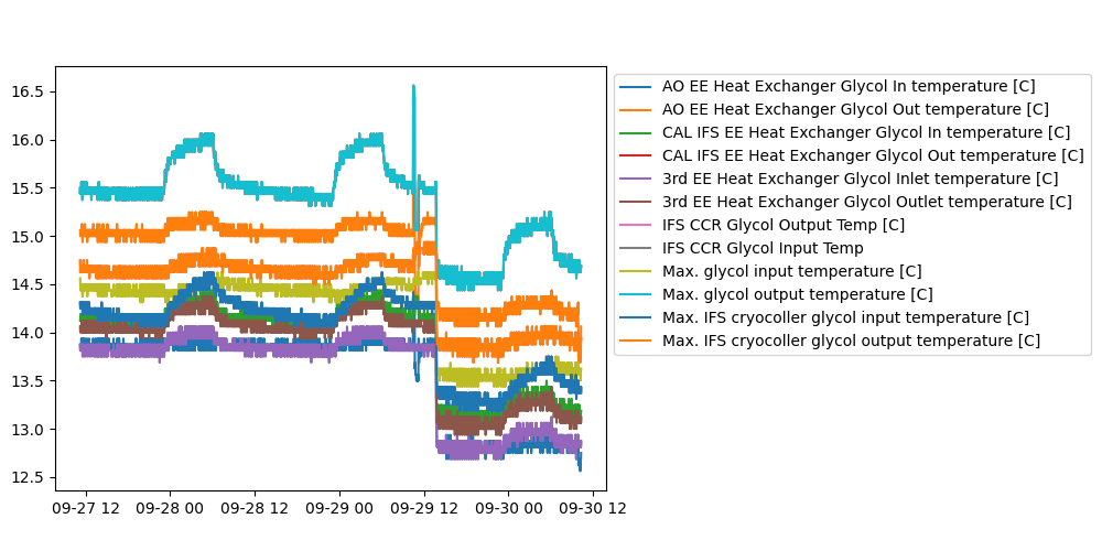
Fig. 2 oneWire logs for all keys matching query ‘glycol’ over a period of 3 days.

Sending Commands

Inasmuch as possible, gpilib2 command names are standardized. All individual components (where relevant) will have init, datum, and sim methods. All collections of components (i.e., coronagraph, etc.) will have init_all and datum_all methods. All components and collections of components will have move methods. The particular syntax of each move command will vary in the allowed keywords, and can be looked up in this documentation, or by printing the docstring of a particular command from within an interactive ipython session, for example:

gpi.coronagraph.move?

Queueing Commands

All commands sent through the rpc object can be executed immediately (via the execute() method) or queued (by passing queue=True to the same method) for later execution (via the execute_queue() method). Every move command for all objects accepts a boolean queue input keyword argument.

Execution of a queue involves issuing all pending commands in the queue asynchronously (such that they are executed as quickly as possible). Both single command execution and queue execution will check on the ack status of the command, and raise RunTimeError exceptions if any errors are encountered in issuing any of the commands.

By default, both single command execution and queue execution will not return until the GMB status variable for the command (or all commands in the queue) shows completion or error. In the case of errors, a RunTimeError exception will be raised. If keyword input nowait is set, then both execute() and execute_queue() will return immediately after checking for a successful ack.

Warning

The nowait and queue keywords are primarily intended for use in higher-level functionality where specific sequences of parallel execution have been well mapped out. They are not recommended for ordinary interactive use of low-level move methods, unless you really, really know what you’re doing.

In addition to their move commands, many of the gpi sub-objects have utility wrappers allowing for easier commanding of standardized move settings. For example, all components of source have an extract() and deploy() method to extract and deploy the ASU and CAL Sphere, and turn their attenuation (and, in the case of the ASU, the SC power) down and up, respectively.